A while ago I wanted to explore my career options so I did a bit of interviewing for various companies. In one of the technical interviews, I was tasked to analyse a dataset and build a predictive model. Noticing that the target variable was ordinal, I decided to build an ordinal regression model using a Bayesian approach. Now, I’m guessing ordinal regression, and Bayesian methods, aren’t that well known, because the interviewers were completely unfamiliar and somewhat sceptical. Needless to say, that particular company did not offer me a position. I think more people should be aware of both ordinal regression and Bayesian methods, so here is a write up on the approach.
The code to fit a model and reproduce the plots is available on GitHub.
The wine dataset
The dataset used for this model is a wine dataset, comprising a set of objective measurements (acidity levels, PH values, ABV, etc.), and a quality label set by taking the average of three sommeliers' scores. There are quite a few columns in the dataset, as can be seen in the scatterplot below. There are 1599 red wines and 4898 white wines, distinguished by colour.
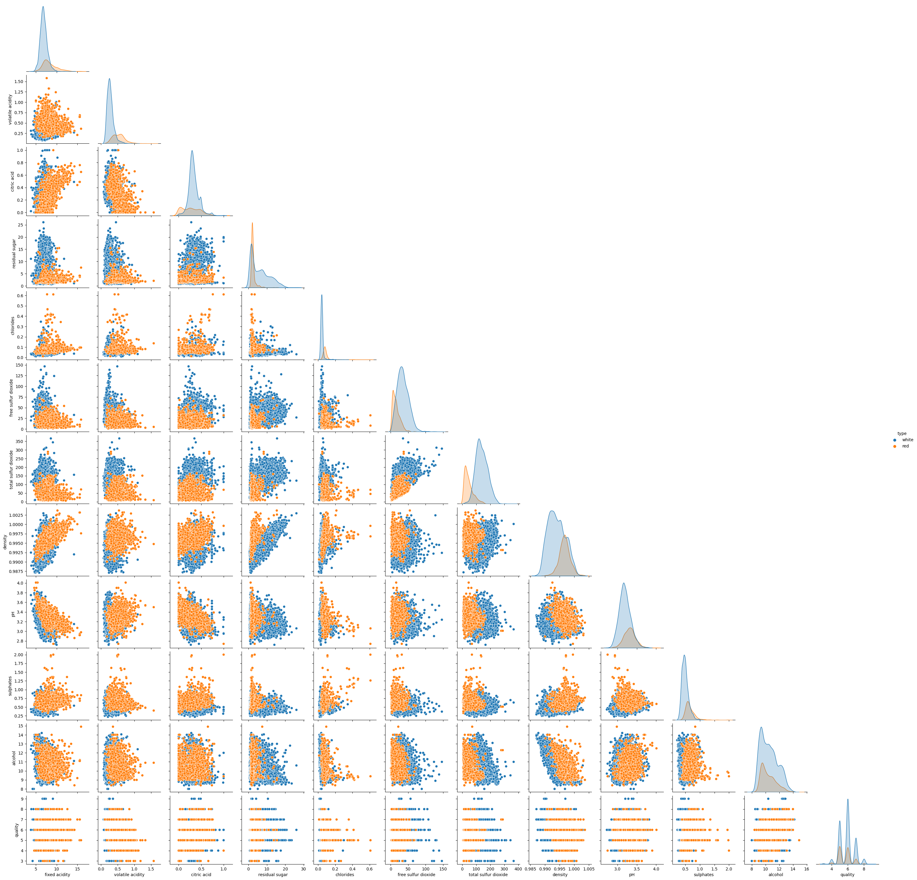
Figure 1: Scatterplot of the wine features. You might want to right-click and ‘open in new tab’ to see anything.
The quality labels are integers ranging from 3 to 9, with most wines scoring around 6. After hearing this, you might say “But those are numbers! Why not use a regular regression model?”. You absolutely could, but such a model assumes that the ‘distance’ between consequtive scores is always the same. Lets unpack that statement.
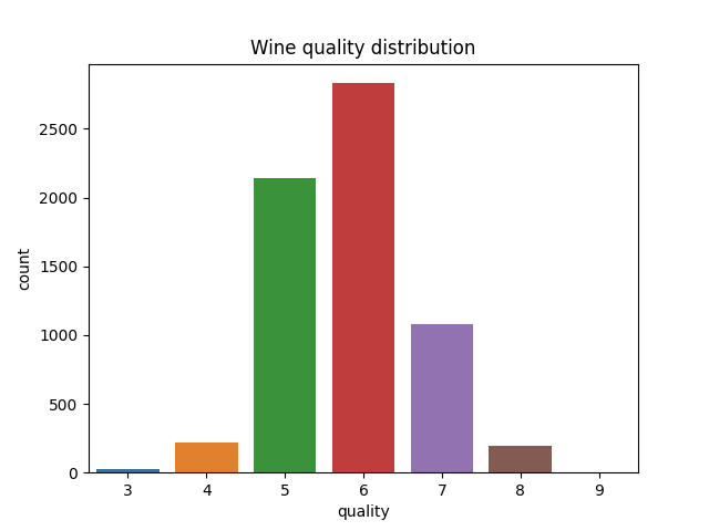
Figure 2: Bar plot of the quality label distribution.
We observe the quality of wine through the judgement of sommeliers, not the quality directly. It is conceivable that the quality difference between wines rate e.g. 3 and 4 might be smaller than between wines rated 6 and 7. Perhaps you are familiar with IMDB and its ratings. Everything below ~7 is often mediocre or outright bad, while the quality difference between 7 to 8 is often substantial. The ordinal regression model lets us model these differences in addition to predicting the quality score itself, which creates a much richer model for our data.
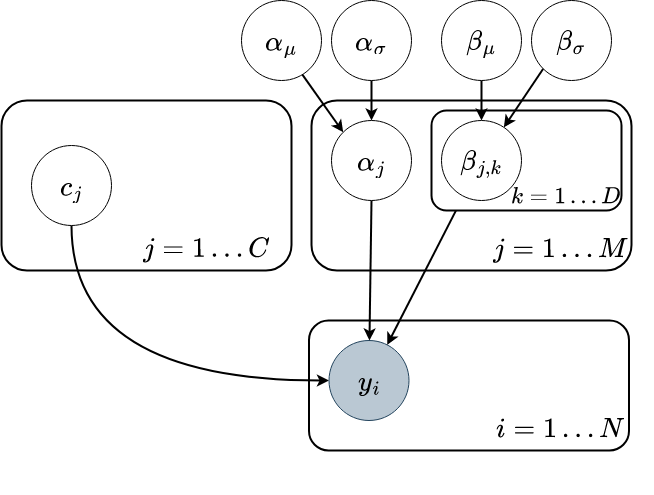
A Bayesian Ordinal Regression model
So how is this model implemented? In a nutshell, it has a regular regression component, and a parameter vector called cutpoints, which is how the difference between scores is modelled. These two components are combined in a OrderedLogistic likelihood, which works by running the regression in log-odds-space, using the cutpoints to separate the value into the various categories. The whole thing is a bit like a partitioned logistic function. There are already very good resources and visualisations out there and I encourage you to give this statistical rethinking lecture a watch, or this blog post a read for more details.
For our data, we are going to build a hierarchical model, allowing partially pooled intercepts and weights for red and white whine. This only affects the regression part.
We use numpyro to implement our model. It takes feature matrix X, a vector of wine type indices t, and target quality y.
Here we refer to the number of target labels as nclasses.
def ordinal_regression(X, t, ntypes, nclasses, anchor_point=0.0, y=None):
    N, D = X.shape

    # intercept hyperpriors
    alpha_loc = npo.sample("alpha_loc", dist.Cauchy(0, 1))
    alpha_scale = npo.sample("alpha_scale", dist.HalfCauchy(1))

    # slopes hyperpriors
    beta_loc = npo.sample("beta_loc", dist.Cauchy(jnp.zeros(D), 1)).reshape(-1, 1)
    beta_scale = npo.sample("beta_scale", dist.HalfCauchy(jnp.ones(D))).reshape(-1, 1)

    # regression component
    with npo.plate("type", ntypes, dim=-1):
        alpha = npo.sample("alpha", dist.Normal(alpha_loc, alpha_scale))

        with npo.plate("dim", D, dim=-2):
            beta = npo.sample("beta", dist.Normal(beta_loc, beta_scale))

    # cutpoints
    with npo.handlers.reparam(config={"c": TransformReparam()}):
        c = npo.sample(
            "c",
            dist.TransformedDistribution(
                dist.Dirichlet(jnp.ones((nclasses,))),
                dist.transforms.SimplexToOrderedTransform(anchor_point),
            ),
        )

    # likelihood
    with npo.plate("obs", N):
        eta = alpha[t] + jnp.sum(X.T * beta[:, t], 0)
        npo.sample("y", dist.OrderedLogistic(eta, c), obs=y)
Analysing the data
After fitting the model using MCMC we can use it to analyse the data. Before we use the model to draw any conclusions we validate that it captures the data well with a posterior predictive check.
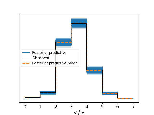
Figure 3: Posterior prediction check. The predictions capture the emprical distribution nicely.
Behind the scenes I have also checked effective sample size, R-hat, and trace plots, and they look good. We can now look at e.g. feature importance by looking at the posterior betas.
![Figure 4: Feature importance (in log-odds). Betas are indexed [feature number, wine type]. A wine type of 0 means white, and 1 means red.](/ox-hugo/posterior_betas.png)
Figure 4: Feature importance (in log-odds). Betas are indexed [feature number, wine type]. A wine type of 0 means white, and 1 means red.
There are plenty of insights to find here. For instance, we see that having high density (feature 7) negative impacts quality (this is especially noticable for white wine). We also see that alcohol (feature 10) has a positive effect (higher for red wine) on quality.
Feature importance could be computed with a regular linear regression, but since we used an ordinal model we can also plot the posterior cutpoints. These reveal that the biggest leap in quality happens between quality scores 5 and 6. Scores above 6 are not systematically different, and the same is true for scores below 5.
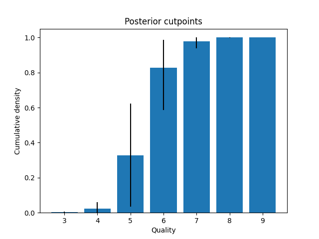
Figure 5: Posterior cut points with 0.95 HPDI as black bars. The biggest increase in underlying quality happens between quality scores 5 and 6.
Closing remarks
After reading this you hopefully see the value of ordinal regression models. If the target variables are ordinal, they should be preferred to linear regression models, as they allow for varying ‘distance’ between target labels, while ensuring correct ordering. Using this with probabilistic programming languages such as numpyro is straightforward and very flexible.
As always, the code is available on GitHub. Thanks for reading!