The data frame is the workhorse of anything related to data and is an incredibly flexible tool. It can be used for almost everything: organising, filtering, transforming, plotting, etc. In this article we are going to see that it is probaly even more flexible than people think!
Good old data frames
When you think of data frames you might be thinking of something square with numbers in it. Perhaps something like
julia> df = DataFrame(
           transaction_id=1:6,
           customer_id=[1, 1, 2, 2, 2, 3],
           amount=[2, 3, 1, 4, 5, 9],
       )
6×3 DataFrame
 Row │ transaction_id  customer_id  amount
     │ Int64           Int64        Int64
─────┼─────────────────────────────────────
   1 │              1            1       2
   2 │              2            1       3
   3 │              3            2       1
   4 │              4            2       4
   5 │              5            2       5
   6 │              6            3       9
Upon seeing the output above you might feel a strong urge to compute summary statistics so you can report them to your stakeholders.
If you do, you might reach for split-apply-combine strategies. These are commonly implemented as a grouping operation, followed by a transformation and a way to aggregate the results.
In DataFrames.jl we can compute the mean amount bought by customers by running
julia> combine(groupby(df, :customer_id), :amount => mean => :amount_mean)
3×2 DataFrame
 Row │ customer_id  amount_mean
     │ Int64        Float64
─────┼──────────────────────────
   1 │           1      2.5
   2 │           2      3.33333
   3 │           3      9.0
Cool. Now you can send the above figures to your stakeholder and leave early for the day. But what if we wanted to do something more interesting?
Beyond boring numbers
Consider a situation where we have gathered data from multiple sub-populations and we want to analyse them in isolation. They could be groups by region, company, gender etc. For this example let us consider time series (inspired by a recent real life use case of mine).
t = float.(1:100)
random_walk(t; x0, σ) = x0 .+ cumsum(map(i -> σ*randn(rng), t))
df = DataFrame(
    :t  => t,
    :y1 => random_walk(t; x0=1, σ=0.1),
    :y2 => random_walk(t; x0=-1, σ=0.15),
    :y3 => random_walk(t; x0=0.5, σ=0.25),
)
df = stack(df, Not(:t))
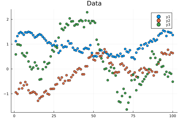
Figure 1: Three different time series we want to analyse.
We are now interested in how these time series evolve. Since they are not correlated we want to model them independently and then use the models to produce forecasts.
Split-apply-machine-learning
Let us break the problem down into pieces and focus on training a model first. Gaussian processes (GPs) are powerful models when dealing with temporal data so let us write a function to train one. The function will take a data frame, fit a GP and then return it.
function fit_model(df)
    t = df.t
    y = df.value
    signal = first(df.variable)
    kernel = SE(0.0, 0.0)
    gp = GP(t, y, MeanConst(mean(y)), kernel, log(0.5))
    optimize!(gp)
    gp
end
Great, now we can plug in our data and get a GP back.
But we said we wanted to do this for each time series, so we have to split the data into groups, maybe loop over the different groups and then apply fit_model.
You know, this sounds very similar to what we did before in the toy example.
Thinking a bit more about it, we have just replaced “compute a summary statistic” with the somewhat more abstraction notion of “fit a model and forecast into the future”.
Here is a wild idea: What if we simply replace the call to mean in our split-apply-combine code from above with calls to fit_model?
# we are also using AsTable(:) instead of a single column name below
julia> models = combine(groupby(df, :variable), AsTable(:) => fit_model => :model)
3×2 DataFrame
 Row │ variable  model
     │ String    GPE…
─────┼─────────────────────────────────────────────
   1 │ y1        GP Exact object:\n  Dim = 1\n  N…
   2 │ y2        GP Exact object:\n  Dim = 1\n  N…
   3 │ y3        GP Exact object:\n  Dim = 1\n  N…
Hey, It Just Works™! The data frame knows how to deal with foreign data types such as GPs just fine and can without trouble store them.
We can now access the GPs by looping over the rows corresponding to each group models[i,:model], then we apply a function to forecast…
But wait. Isn’t this the exact same problem again? Only this time we are looking at an already-transformed data frame.
Hmm. If we had a function plot_fit to plot forecasts…
# for the examples below fit_model is updated to return (gp, t, y, signal)
# note that plot_fit accepts a tuple instead of splatting the arguments
function plot_fit((gp, t, y, signal); forecast=10)
    t_pred = vcat(t, t[end]:t[end] + forecast)
    μ, Σ = predict_y(gp, t_pred)
    plt = plot(t_pred, μ, ribbon=2*sqrt.(Σ), label=nothing)
    plt = scatter!(plt, t, y, title=signal, label=nothing)
    return plt
end
… could it really be as simple as composing it with fit_model ?
N = length(unique(df.variable))
plots = combine(groupby(df, :variable), AsTable(:) => plot_fit ∘ fit_model => :plot)
fit_plt = plot(plots.plot..., layout=(N, 1), size=(600, 200N))
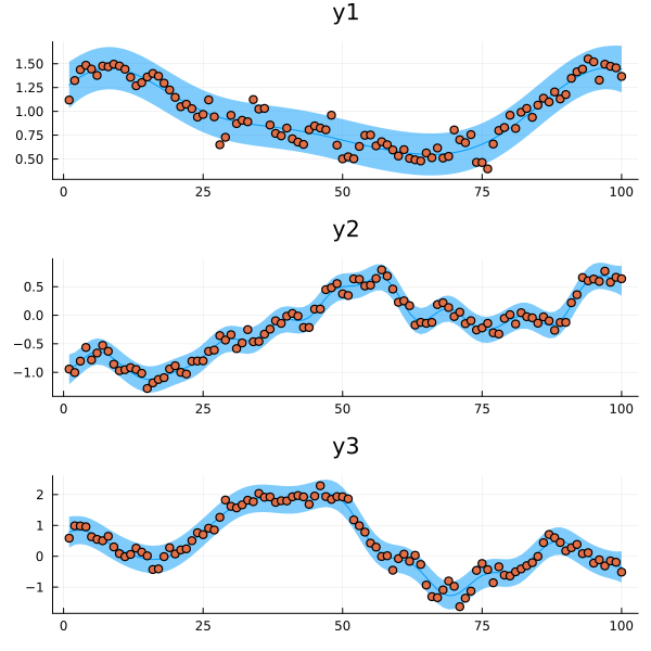
Figure 2: The resulting models fitted to the individual time series.
Cool! Our entire analysis is running inside the split-apply-combine framework!
Closing remarks
Hopefully by now you see the true potential of split-apply-combine:
Any computation that takes a dataframe can be plugged into this framework, we are not limited to functions that produce summary statistics.
And since everything composes so nicely in Julia we are able to produce and store data types from packages completely unrelated to DataFrames.jl
without losing performance.
Thank you for reading! If you want to reproduce the plots the code is available on my GitHub.