Weather forecasting is a tricky problem. Traditionally, it has been done by manually modelling weather dynamics using differential equations, but this approach is highly dependent on us getting the equations right. To avoid this problem, we can use machine learning to directly predict the weather, which let’s us make predictions without modelling the dynamics. However, this approach requires huge amounts of data to reach good performance. Fortunately, there is a middle ground: What if we instead use machine learning to model the dynamics of the weather?
Instead of trying to model how the weather will look in the next time step, what if we instead model how the weather changes between time steps? More concretely: What if we learn the differential equations that govern the change in weather? In this blog article we are going to use Julia and the SciML ecosystem to do just that. We are going to see how neural ordinary differential equations (neural ODEs) relate to “regular” networks, how to train them and see how they can extrapolate time series from just a tiny amount of training data.
Neural ODEs for time series
To start us off, let’s talk about how neural ODEs are used for time series modeling. Recall that in a standard machine learning setting we would assume a discrete set of observations \(y_0, y_1, \dots y_k, \) \( y_i \in \mathbb{R}^n \) at time points \(t_0, t_1, \dots t_k, \), \(t_i \in \mathbb{R} \) to be related through some function \( y_i = f(t_i; \theta) \) where \( \theta \) are learnable parameters. However, in a neural ODE we consider a continuous setting and instead assume that the change in \(y\) is governed by an ODE
\[ \frac{\partial y}{\partial t} = f(y; \theta). \]
The goal is hence not to learn the relationship between \(y\) and \(t\), but the underlying dynamics of change. If the dynamics do not change too much, this has very powerful generalisation capabilities. It is helpful to think of this formulation as “a neural network inside an ODE” or maybe “an ODE with learnable parameters”. In fact, the “forward pass” through a neural ODE is equivalent to solving an initial value problem, where \( y(t_0) \) is the input features and we replace hand-crafted equations with a neural network. This means that a single forward pass gives us an entire trajectory in contrast to e.g. RNNs, where each forward pass through the model gives a single prediction in time.
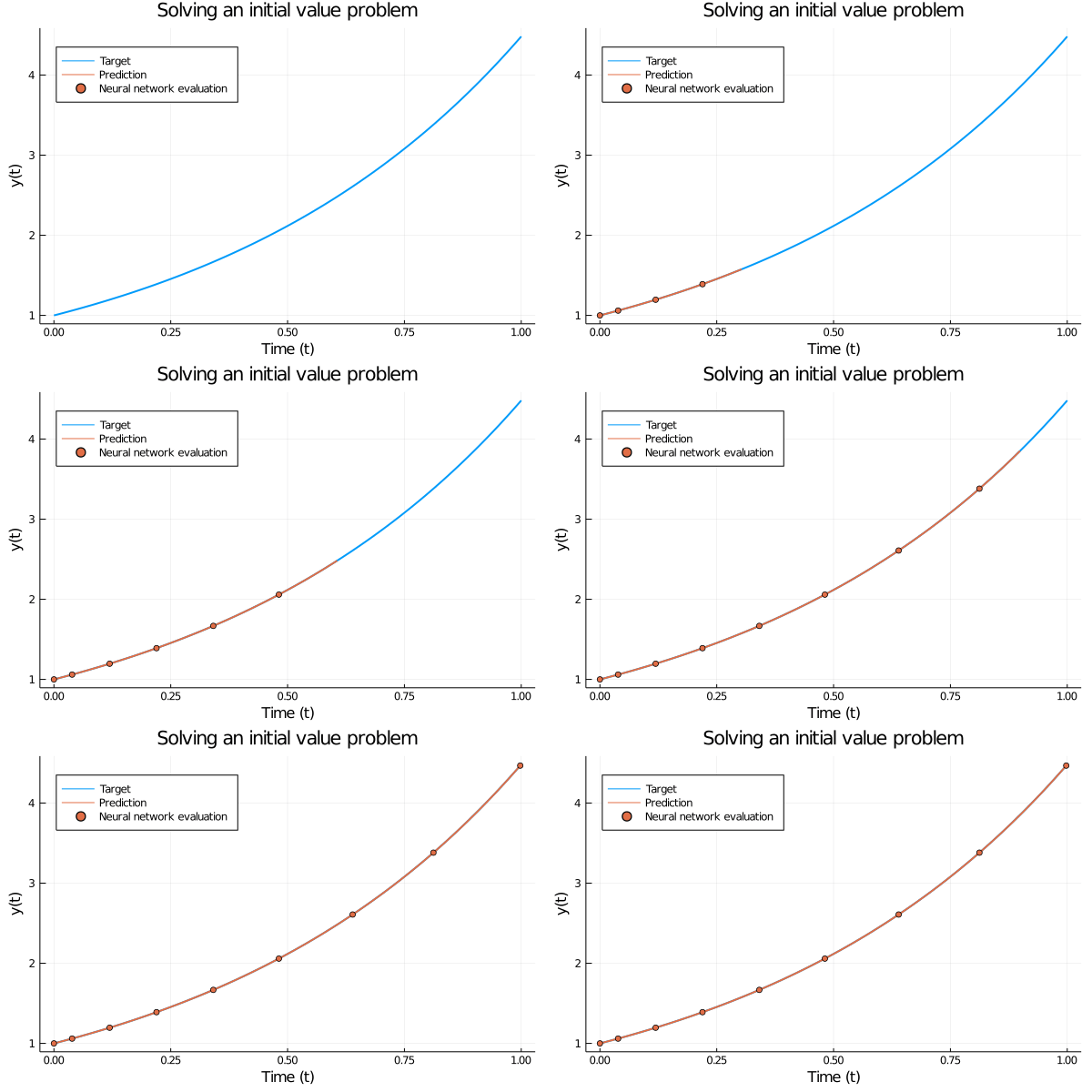
To make this more concrete, consider a forward pass for \(y(t_0) = 1.0\) where the model has been trained on \(f^{\star}(y) = \exp(1.5y)\). The forward pass consist of inputting \(y(t_0)\) and using an ODE solver to step forward in time to solve \[ y(t) = y(t_0) + \int_{t_0}^t \frac{\partial y}{\partial t} \partial t = y(t_0) + \int_{t_0}^t f^{\star}(y(t)) \partial t, \] where we use a neural network to model \(f^{\star}\).

Figure 1: Solving a simple initial value problem using a trained neural ODE. The only difference from a “regular” initial value problem is that the ODE is governed by a neural network instead of a hand-crafted set of equations. The trained network accurately follows the analytic solution.
So how do we train a network inside an ODE? As long as we can
take gradients of \(\theta\) with respect to the loss we can train it
using standard gradient based methods. Fortunately,
DiffEqFlux.jl takes care of everything required to do this for us.
There are several strategies that can be specified to compute
gradients, and depending on
the problem you might prefer one over the other. However, for this article
the default InterpolatingAdjoint will be perfectly fine.
Model implementation
Now that we have a good conceptual idea of the model, let’s see it
in practice. We are going to use DiffEqFlux.jl to do the heavy lifting, which combines the ODE
solvers of DifferentialEquations.jl with the differentiable
programming capabilities of Flux.jl. Using DiffEqFlux, we can simply
construct a neural network to model \(f\) and plug that into a NeuralODE
object. The NeuralODE object itself has a few additional important
hyper-parameters though. Firstly, we have to specify an ODE solver and a time span to
solve on. We will use the Tsit5 solver, which uses an explicit
method. Secondly, the parameters reltol and abstol let us configure the solution
error tolerance to trade off accuracy and training time.
Recall that a forward pass means solving an initial value problem,
hence a lower tolerance gives a more accurate solution, and in turn
better gradient estimates. But of course, this requires
more function evaluations and are consequently slower to compute.
  using DiffEqFlux

  function neural_ode(t, data_dim; saveat = t)
      f = FastChain(FastDense(data_dim, 64, swish),
                    FastDense(64, 32, swish),
                    FastDense(32, data_dim))

      node = NeuralODE(f, (minimum(t), maximum(t)), Tsit5(),
                       saveat = saveat, abstol = 1e-9,
                       reltol = 1e-9)
  end
The Delhi dataset
The dataset we are going to use comprises daily measurements of the climate in Delhi over several years. The entire dataset is a single time series, where the last part is set aside for testing. We will combine both the train and test set though, since we won’t even need half of the training set to fit a good model. Let’s load up the data and visualize it.
  using DataFrames, CSV
  delhi_train = CSV.read("data/timeseries/dehli-temp/DailyDelhiClimateTrain.csv")
  delhi_test = CSV.read("data/timeseries/dehli-temp/DailyDelhiClimateTest.csv")
  delhi = vcat(delhi_train, delhi_test)
Figure 2: Visualisation of the raw data. There is a clear seasonal trend, but there are some extreme outliers among the pressure measurements, which make it difficult to see any patterns.
Something is off with the air pressure measurements, indicated by the extreme outliers after 2016. However, prior to 2016 the measurements show a nice periodic behavior.
Figure 3: Zooming in on the pressure before 2016 reveal the same pleasant seasonal behavior as in the other measurements.
As an aside, if you read the dataset description it claims that the Mean pressure
variable is measured in atm. Now, I have never been to Delhi, but I have my doubts since that would
mean that the city of Delhi suffers under a thousand atmospheres
worth of pressure. While such a phenomenon would be pretty cool and without a doubt get
scientists excited, I think it is more likely the units simply got
mixed up. Based on that, I have chosen to present the data in
hectopascal, which is commonly used in meteorological forecasts
instead of using its documented unit. Anyway, let’s prepare the data for model training.
Data pre-processing
All the metrics vary a lot from day to day, so to emphasis the overall trend in the data we will average the observations into months.
  using Statistics
  using Base.Iterators: take, cycle

  delhi[:,:year] = Float64.(year.(delhi[:,:date]))
  delhi[:,:month] = Float64.(month.(delhi[:,:date]))
  df_mean = by(delhi, [:year, :month],
               :meantemp => mean,
               :humidity => mean,
               :wind_speed => mean,
               :meanpressure => mean)
  rename!(df_mean, [:year, :month, :meantemp,
                    :humidity, :wind_speed, :meanpressure])

  df_mean[!,:date] .= df_mean[:,:year] .+ df_mean[:,:month] ./ 12;
In addition to averaging, we will normalize the data. The features are normalized to have zero mean and unit variance, and the temporal dimension is shifted to start at \(0\). Finally, we take the first \(20\) observations as our training data and leave the remaining for testing.
  features = [:meantemp, :humidity, :wind_speed, :meanpressure]

  t = df_mean[:, :date] |>
      t -> t .- minimum(t) |>
      t -> reshape(t, 1, :)

  y = df_mean[:, features] |>
      y -> Matrix(y)' |>
      y -> (y .- mean(y, dims = 2)) ./ std(y, dims = 2)

  T = 20
  train_dates = df_mean[1:T, :date]
  test_dates = df_mean[T+1:end, :date]
  train_t, test_t = t[1:T], t[T:end]
  train_y, test_y = y[:,1:T], y[:,T:end];
Figure 4: The normalized data split into test and train. This is what the model will “see” during training and evaluation.
Since we are training our model using gradient descent, we run the risk of getting stuck into a bad local minima. This is particularly true when training on a periodic time series, since the model can easily settle with predicting the time series mean. Mini-batching can be used to mitigate this, but for this problem we are going to employ a different method. We are going to train on the first couple of observations until convergence, then introduce a few more observations. Then train until convergence, introduce some more observations, etc… By doing this, we let the model adapt to local changes, resulting in a better fit. The code below implements this training procedure.
  using OrdinaryDiffEq, Flux, Random

  function train_one_round(node, θ, y, opt, maxiters,
                           y0 = y[:, 1]; kwargs...)
      predict(θ) = Array(node(y0, θ))
      loss(θ) = begin
          ŷ = predict(θ)
          Flux.mse(ŷ, y)
      end

      θ = θ == nothing ? node.p : θ
      res = DiffEqFlux.sciml_train(
          loss, θ, opt,
          maxiters = maxiters;
          kwargs...
      )
      return res.minimizer
  end

  function train(θ = nothing, maxiters = 150, lr = 1e-2)
      log_results(θs, losses) =
          (θ, loss) -> begin
              push!(θs, copy(θ))
              push!(losses, loss)
              false
          end

      θs, losses = [], []
      num_obs = 4:4:length(train_t)
      for k in num_obs
          node = neural_ode(train_t[1:k], size(y, 1))
          θ = train_one_round(
              node, θ, train_y[:, 1:k],
              ADAMW(lr), maxiters;
              cb = log_results(θs, losses)
          )
      end
      θs, losses
  end

  Random.seed!(1)
  θs, losses = train();

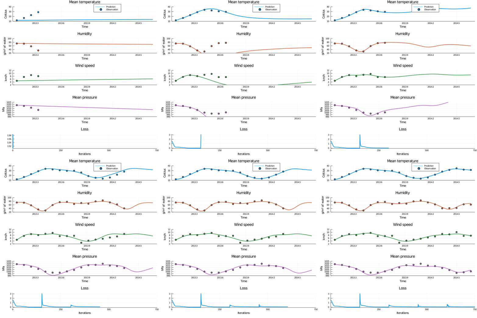
Figure 5: Animation of training through incrementally adding observations. When new observations are added the loss curve makes a sudden jump, but quickly settles down again. This process successfully avoids bad local minima and results in a very nice fit.
The model trains in a minute or two and fits nicely to the training data. Of course, a more interesting question is whether the model generalises or not. To find out we solve the initial value problem for \(f\) with trained parameters and extrapolate into the future.
Figure 6: Forecasting using the trained model. The model has picked up on the seasonality in the data and successfully extrapolates. The final observations are somewhat irregular, and not perfectly captured by the model.
Plotting the predictions show the model has successfully learned the dynamics in the training data and does a really good job extrapolating. Recall that the model was only presented with the first observation in prediction time.
Ending notes
In this article we took a look at neural ODEs and how to use them for time series modelling in Julia. They are a very cool class of models, and while they really shine when modeling physical systems or time series, they are of course not a silver bullet. However, I only covered half the story of neural ODEs in this article. Remember how I talked about them as “neural networks in ODEs”? It turns out that there is nothing stopping us from doing the opposite and plugging an ODE inside a neural network, or using an ODE as stand-alone function approximator. In fact, this has proven particularly useful in normalizing flows, since ODEs naturally model homeomorphisms.
Not being able to model arbitrary functions is both a strength and a weaknesses. Because of this, ODEs come with a very strong inductive bias, which is how they can extrapolate from so little data. That is not to say they are inexpressive though. In fact they can be used as universal function approximators much like fully connected networks through augmented neural ODEs.
Finally I would like to touch upon the amount of knobs and dials to tweak when training neural ODEs. While the neural network used to model the dynamics does not have to be particularly large, we still have the regular parameters to worry about such as network architecture, batch size and learning rate. In addition, we now have to worry about which ODE solver we use, the stiffness of the system, and which sensitivity algorithm we use. While neural ODEs combines the best from differential equations and differentiable programming, it is important to remember that it also combines the complexities.
Thank you for reading! Let me know if you have any questions or comments.