In a previous article we talked about how to put neural networks inside ODEs to learn their dynamics from data. Armed with that knowledge we created a powerful weather forecasting model. But learning the dynamics of a process is only one side of the neural ODE story, they can also be used as very flexible function approximators much like regular neural network. In this article we are going to create continuous neural network layers using neural ODEs and see how they can be used to classify the Fashion MNIST dataset.
The two sides of neural ODEs
Before we get into the implementation, let us take a moment to talk about the differences between using neural ODEs to model evolving processes and as function approximators. ODEs always deal with continuous things, typically evolving over time, but we will see that we can interpret the temporal aspect differently depending on our use case.
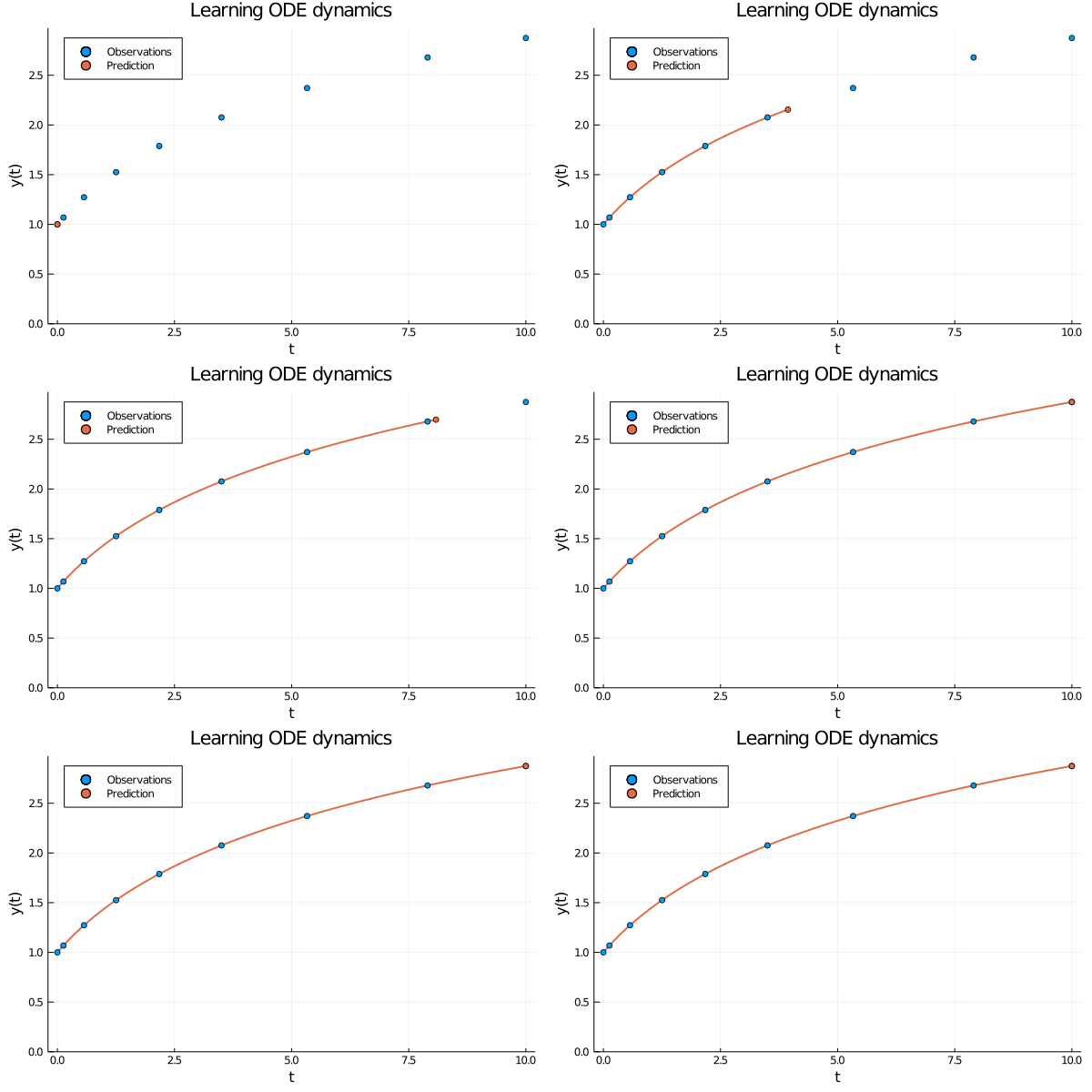
When modelling an evolving process we observe \( (t_0, y_0), (t_1, y_2) \dots (t_N, y_N) \) related through the initial value problem \[ y_i = y_0 + \int_0^i \frac{\partial y}{\partial t} \partial t = y_0 + \int_0^i f(y(t)) \partial t , \] where the dynamics \(f\) is modelled with a neural network. In other words, all observations are generated by the same process and we use a neural network to learn the dynamics of this process.

Figure 1: When using neural ODEs to learn the dynamics of an evolving process all the observations are assumed to be produced by the same trajectory.
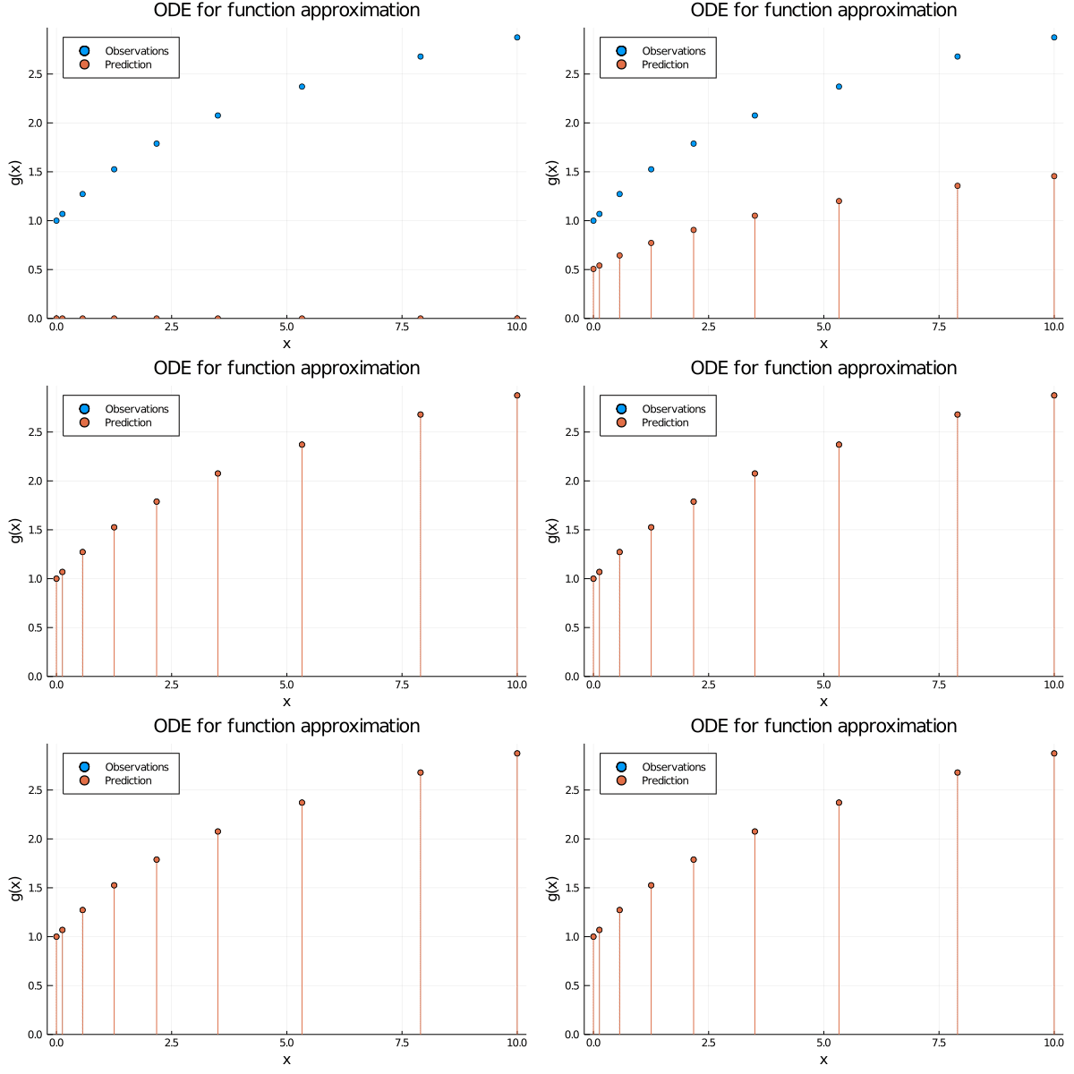
In contrast, when using neural ODEs for function approximation, we observe \( (x_0, y_0), (x_1, y_1) \dots (x_N, y_N) \) related through a mapping \( y_i = g(x_i) \). Indeed, this is the same view as when using a regular neural network. But where is the temporal aspect in this setting? Consider the ODE \(u\prime = f(u(t))\) and initial condition \(u(t) = x_i\) and observed value \( u(T) = y_i \) for some \(T\). If we solve this initial value problem we get a trajectory that smoothly transforms \(x_i\) into \(y\) over the time span \([0, T]\). This means we can express \(g\) as
\[ y_i = g(x_i) = u(0) + \int_0^T \frac{\partial u}{\partial t} \partial t = x_i + \int_0^T f(u(t)) \partial t. \]
In other words, by learning the dynamics we get a continuous transformation where the output of \(g\) evolves over time. The authors of Neural Ordinary Differential Equations liken this to a composition of infinitely many layers in a ResNet model.

Figure 2: When using neural ODEs for function approximation each observation (x_i) induce their own initial value problem, which solutions recover the function value (g(x_i)) at time point (T).
Hopefully Figures 1 and 2 convey the difference between the two perspectives. But before we get to the code, let us peek inside an ODE layer and see what is actually happening.

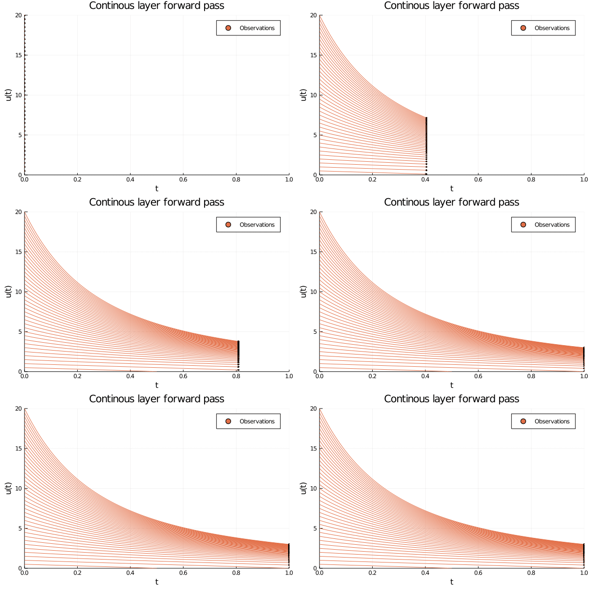
Figure 3: The inside of an ODE layer modelling (y = ln(x)). The initial conditions are given by the data (u(0) = x), which are smoothly transformed into ( u(T) = ln(x)) at (T = 1.0). Observe that the y-axis shows the value of both the input and the output of the layer, and the observations should be thought of as entering the layer on the left side and exiting on the right side.
Neural ODEs for image classification
Now that we have built up some intuition for how continuous layers work, let us put them to use in a neural network and classify the Fashion MNIST dataset. To this end we are going to use the wonderful Julia language. In particular, we are going to use the Flux.jl package for our neural network needs and the DifferentialEquations.jl and DiffEqFlux.jl packages from the SciML ecosystem for the ODE solving. Let us begin with a function to create data loaders. The only pre-processing required of us is that we add an explicit channel dimension to the data.
  using MLDatasets, Images
  using Flux.Data: DataLoader
  using Flux: onehotbatch

  function dataloader((X, y); batchsize, kwargs...)
      addchannel(x) = begin
          W, H, N = size(x)
          reshape(x, W, H, 1, N)
      end
      DataLoader(Float32.(addchannel(X)),
                 Float32.(onehotbatch(y, 0:9)),
                 batchsize = batchsize; kwargs...)
  end
With that out of the way, let us move on to the model. It comprises a single
convolutional layer followed by an ODE layer and
a linear projection to our output logits. In other words, the
ODE layer will do all the heavy lifting after the initial
convolution.
The ODE layer itself is implemented using the
NeuralODE constructor, which takes a neural network dudt modeling the
dynamics, a time span tspan to solve on and an ODE solver (we will use
Tsit5).
We are going to solve over the time span \([0.0, 1.0]\), and since we only
care about final values we will not save any additional function
evaluations that the ODE solver makes. Finally we will train the model
(including the ODE dynamics!) on a GPU, so we move all the model pieces
onto a graphics card using the gpu function.
  using Flux, DiffEqFlux, OrdinaryDiffEq, CUDA
  using Flux: onecold, logitcrossentropy
  CUDA.allowscalar(false)

  function conv_node(;data_dim = 1,
                     num_classes = 10,
                     tspan = (0.f0, 1.f0))
      ode_dim = 2028
      conv = Conv((3, 3), data_dim => 3, relu) |> gpu

      dudt = Chain(Dense(ode_dim, 16, relu),
                   Dense(16, 16, relu),
                   Dense(16, ode_dim, relu)) |> gpu

      node = NeuralODE(dudt, tspan, Tsit5(),
                       reltol = 1e-3, abstol = 1e-3,
                       save_everystep = false,
                       save_start = false) |> gpu

      toarray(x) = reshape(gpu(x), size(x)[1:2])
      classifier = Dense(ode_dim, num_classes) |> gpu
      Chain(conv, flatten, node, toarray, classifier)
  end
With the model and the data in place, we can write our training logic quite succinctly.
  using Statistics: mean
  using Printf

  function train(model, traindata, testdata, opt)
      accuracy(x, y) = mean(onecold(cpu(model(gpu(x)))) .== onecold(y))

      loss(x, y) = begin
          ŷ = model(gpu(x))
          Flux.logitcrossentropy(ŷ, gpu(y))
      end

      callback() = begin
          testloss = mean(b -> loss(b...), testdata)
          testacc = mean(b -> accuracy(b...), testdata)
          @printf "Loss: %1.2f | Accuracy: %1.2f\n" testloss testacc
      end

      @Flux.epochs 1 Flux.train!(
          loss, params(model), traindata, opt;
          cb = Flux.throttle(callback, 25)
      )
  end

  opt = ADAMW(1e-2)
  model = conv_node()
  trainloader = dataloader(FashionMNIST.traindata();
                           batchsize = 128, shuffle = true)
  testloader = dataloader(FashionMNIST.testdata();
                          batchsize = 1024);
  train(model, trainloader, testloader, opt)
Before we move on to look at the training results, let us take a breather and think about an interesting question. How deep is our model? How many layers does it have? The answer is not obvious. We probably agree the convolution layer counts as one layer, and the output projection clearly counts as one. But is it fair to count a continuous ODE layer as a single layer? To answer this question we have to think about how we solve ODEs.
The depth of ODE layers
When solving an ODE, the most important factor that affects compute time is how many times the ODE solver needs to evaluate \(y\prime(t)\), so naturally we want to take large steps between evaluations from an efficiency perspective. However, if we take too large steps, the solution will be inaccurate and of no use to us. It is the ODE solvers task to strike a good balance to efficiently provide an accurate solution. The No free lunch theorem applies to ODE solving just as much as it does to machine learning, so there are quite a few solvers to pick from, and the one we chose will determine how many times \(y\prime(t)\) is evaluated. Put in the context of ODE layers: the solver determines how many times we evaluate \(y\prime(t)\) during a forward pass. Since \(y\prime(t)\) is modeled with a neural network it makes sense to think of the depth of ODE layers as the number of function evaluations the ODE solver needs to make. If you are familiar with RNNs, this is similar to how they are evaluated for each time step. But instead of the output depending on a hidden state it depends on the current \(y\). And when using an RNN we get to decide how many times we recurse, but with ODE layers we are handing that job over to the solver.
So the depth of an ODE layer is determined by how many times \(y\prime(t)\) is evaluated by the ODE
solver during a forward pass, which in turn is decided by the solver
(It also depends on the specified error tolerance, reltol and abstol, but that is not too
important right now). That means we should be able to pick a solver,
count the evaluations during a forward pass, and figure out the model
depth, right? Let us move on to the training results to see if this
tactic works.
Figure 4: The model achieves respectable accuracy on the Fashion MNIST dataset after a few minutes of training on a GPU. Curiously, the number of function evaluations made by the ODE solver increases as training progresses.
Our model trains without issues, and eventually reaches \(0.87\)
accuracy. Interestingly, it initially evaluates \(y\prime(t)\) three
times during a forward pass
but the number of evaluations increases as training progresses. What is going on here?
Since we are making gradient updates to the dudt network, the dynamics
change so the solver has to solve a
slightly different problem every forward pass. Indeed, the depth of
our network grows as we train it, which reveals
that the ODE problem grows more and more difficult as we learn better
dynamics.
Ending notes
Neural ODEs are a flexible class of models. In this article we have seen how to use them as continuous layers in neural networks, and built some intuition for what is going on inside them. We also saw that the concept of network “depth” does not apply directly to ODE layers. Their depth is not something we can choose explicitly, it is decided by how many evaluations the ODE solver makes. This depends on the solver we use, but is also dependent on what error tolerance we specify. A lower tolerance will require more function evaluations, and a deeper model.
While neural ODEs introduce additional hyper-parameters they also have several advantages compared to regular networks. One very cool aspect is that we are able to train them using the adjoint sensitivity method, which lets us take gradients without storing the activations during the forward pass. This lets us train with constant memory usage. Additionally, by leveraging an ODE solver the model implicitly learns its depth from data, which can save us the trouble of trying out different architectures. Finally, they can scale to very large problems using very few parameters, as demonstrated by FFJORD for instance.
I hope you enjoyed reading this article. Do not hesitate to reach out to me should you have any question or comments.