In the previous article we were introduced to the Palmer Penguins, their eating habits, and built a recommender system that would serve them their favourite fish. However, the system we built was overly simplistic and assumed a single favourite fish across the population. As we all know, there is no single best of anything. It all comes down to personal preference. In this article we are going to see how to improve the system through contextual multi-armed bandits, which will allow learning the penguins preferences much more granularly than a population average.
This article will use the same setting and data set as the first part, so I highly recommend you give it a read for some additional context, an explanation of the data and a description of the already implemented system.
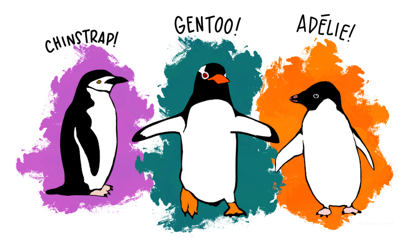
Figure 1: The Palmer penguins are back for more fish. Artwork by @allison_horst.
Measuring the penguins
The greatest weakness of the previous system was that it did not take into account any information about the penguins it was feeding. It was merely trying to choose the most popular fish across the board. A much more powerful approach is to try and learn patterns in the penguins preferences, and identify parts of the population that have similar preferences. If we were to observe the features of approaching penguins, we could decide which fish to feed based on what we know about the preferences of similarly-looking penguins. Fortunately, the engineers of our fish-feeding operation are already hard at work on an improved system equipped with sensors to observe and measure the penguins bill, body mass and flippers. Let us take a look at these features.

Figure 2: The different penguins species have different attributes. For instance, the Gentoo is much heavier than the other species and has much longer flippers.
As we can clearly see, there are significant differences between different penguin species. And all this information can be used to better predict their preferences. To refresh your memory, here is the table of eating habits from the first part (entries indicate probability of eating a fish). Since the different species have quite diverse features and eating preferences, it makes a lot of sense to try and capture this information in the model.
| Adelie | Chinstrap | Gentoo | |
|---|---|---|---|
| Mullet | .50 | .50 | .70 |
| Anchovies | .60 | .95 | .1 |
| Sardines | .15 | .15 | .95 |
If we were planning a real expedition to Antarctica we would of course not know the dietary preferences or the penguins features beforehand. After all, if we knew them we would not need machine learning. However, having seen the data will help us diagnose the algorithm we implement later on.
Contextual Bayesian bandits
Since we already set up the PalmerEnv environment in the first part, let us dive straight into contextual bandits. They are an extension of “regular” bandit problems where the agent is presented with a context before making a decision. In our case the context is the features of the penguin looking for a bite. This setting might remind you of supervised learning, and indeed it is very similar. The key difference is that we do not collect data for batch training; we learn solely from action rewards (We can do batch training as well though. More on this later.).
In the first part we took a Bayesian approach to multi-armed bandits, and since the Bayesian framework is so general, we can reuse a lot of our implementation. The goal is still to infer the posterior over expected rewards \(P(\theta \vert \mathcal{D})\), and we can still use Thompson sampling for selecting actions. However, the Beta-Bernoulli model has to be replaced with something that can take context information into account. Let us replace it with Bayesian logistic regression.
Bayesian logistic regression
In Bayesian logistic regression we model the action success probabilities as \(P(\theta \vert x, \beta) = \sigma(x \beta), \) where \(\sigma\) denotes the logistic function, and we put a Normal prior on the parameters \(\beta \sim \mathcal{N}(\mu_0, \Sigma_0)\). This means we have to compute the posterior predictive distribution to get \(\theta\) which for the logistic model is given by
\[ P(\theta \vert x, \mathcal{D}) = \int \sigma(x \beta) P(\beta \vert \mathcal{D}) d\beta. \]
Unfortunately \(P(\beta \vert \mathcal{D})\) has no closed form solution, so we have to resort to approximations. A commonly used approximation that generally performs well for logistic regression is the Laplace approximation, which is also straightforward to implement.
Since this article is about multi-armed bandits, we will gloss-over the details of Laplace approximations, but we do have to implement it to make progress. In short, we approximate the posterior with a Normal distribution \(\theta \sim \mathcal{N}(\mu, \Sigma)\) where \(\mu\) is given by the posterior mode and \(\Sigma\) is given by the inverse Hessian evaluated at \(\mu\). The following code implements Laplace approximation by using the Optim.jl package to find the posterior mode. One detail worth mentioning is the rounding of the covariance matrix. The MvNormal constructor requires the covariance matrix to be symmetric (not unreasonable), but due to rounding errors, this is not always the case after finding the posterior mode. Rounding to six significant digits is a hack put in there to make sure it is symmetric.
using DataFrames, CSV, HTTP
using Distributions, Statistics, ConjugatePriors
using Plots, StatsPlots, MLDataUtils
using Optim, NLSolversBase

σ(z) = 1 / (1 + exp(-z))

unnorm_log_posterior(x, y, θ, pθ) = begin
    z = σ.(x.*θ)
    log_likelihood = sum(@. y*log(z) + (1 - y)*log((1 - z)))
    log_prior = logpdf(pθ, θ)
    log_likelihood + log_prior
end

laplace(x, y, θ0, pθ) = begin
    obj(θ) = -unnorm_log_posterior(x, y, θ, pθ)
    f = TwiceDifferentiable(obj, θ0; autodiff = :forward)
    μ = optimize(f, θ0) |> Optim.minimizer
    H = hessian!(f, μ)
    Σ = round.(inv(H); sigdigits=6)
    MvNormal(μ, Σ)
end
With that out of the way, we can proceed with implementing the agent. Before doing that though, we will standardise the input features to make life easier for the algorithm. While it is possible to estimate the population mean and variance as new observations come in, we are going to put aside a few observations for estimating these parameters and use the same estimate for all future observations.
observables = [
    :bill_depth_mm,
    :bill_length_mm,
    :body_mass_g,
    :flipper_length_mm
]

seen, unseen = stratifiedobs(x -> x.species, palmer,
                             p = .10, shuffle = true)
observations = Matrix(palmer[:, observables])
seen_x = Matrix(seen[:, observables])
unseen_x = Matrix(unseen[:, observables])
println("Estimating μ and σ from $(size(seen_x, 1)) penguins.")

standardiser(x) = begin
    μ = mean(x, dims = 1)
    σ = std(x, dims = 1)
    x̃ -> (x̃ .- μ) ./ σ
end

standardise = standardiser(seen_x);
Estimating μ and σ from 34 penguins.
We can now create our new and improved agent! It will look very similar to the BetaBernoulli struct we implemented in the last article, but there are some important differences. The BetaBernoulli struct had a Beta distribution for each action, directly modelling \(\theta\), but this time the agent will have a Normal distribution over parameter vectors \(\beta\) per action instead. If we let \(\mathcal{D}_{t} = (a_{1:t}, r_{1:t}, x_{1:t})\) denote the seen actions, rewards and contexts up to round \(t\), a new round is played as follows. First, the agent is provided a context \(x_t\). We then sample \(\hat{\beta}_a \sim p(\beta \vert x_t, \mathcal{D}_{t-1})\) for each action, compute the \(\mathbb{E}[\theta \vert \hat{\beta}_a, x_t, \mathcal{D}_{t-1}]\), and choose \(a\) to maximise the expectation. We then observe a reward and update the posterior over the chosen \(\beta_a\) using the Laplace approximation we implemented earlier.
struct LogisticRegression
    pβ::Array{MvNormal{Float64}}
    standardise::Function
    K::Int
    D::Int
end

LogisticRegression(K, D, standardise) =
    LogisticRegression([MvNormal(randn(D), 1) for _ in 1:K],
                       standardise, K, D)

Base.length(b::LogisticRegression) = b.K
Base.size(b::LogisticRegression) = b.K, b.D

(b::LogisticRegression)(act, context) = begin
    x = standardise(context')
    β = mapreduce(rand, hcat, b.pβ)
    θ = vec(σ.(x*β))
    a = argmax(θ)
    r = act(a)
    b.pβ[a] = laplace(x[:], r, β[:,a], b.pβ[a])
    a
end
Alright, all we need now is a function for running the model. The following snippets are adapted from the last article which have been tweaked to provide the agent with context.
run_with_context(env, agent, oracle, expected_reward, observables; rounds) = begin
    map(1:rounds) do _
        penguin = first(rand(env))
        context = Array(penguin[observables])
        a = agent(fish -> env(fish, penguin), context)
        θ = expected_reward(penguin, a)
        astar = oracle(penguin)
        θstar = expected_reward(penguin, astar)
        ρ = θstar - θ
    end
end
Time to see the model in action! We are going to run it alongside the Beta-Bernoulli model for comparison. As seen in the code, the Beta-Bernoulli model discards context information, which should give us a hint about its performance in relation to the logistic regression model. To be able to compute the regret we use an oracle function which will return the best action for a context.
eat_probs = [
    .50 .50 .70
    .60 .75 .10
    .15 .15 .80
]

rounds = 500
K, D = length.((fishes, observables))
logreg = LogisticRegression(K, D, standardise)
betabern = (act, ctx) -> BetaBernoulli(K)(act)
oracle(penguin) = argmax(eat_probs[:, penguin.species])
eat_prob(penguin, fish) = eat_probs[fish, penguin.species]
env = PalmerEnv(unseen, eat_probs)

logreg_regret = run_with_context(
    env, logreg, oracle, eat_prob, observables; rounds
);
betabern_regret = run_with_context(
    env, betabern, oracle, eat_prob, observables; rounds
);
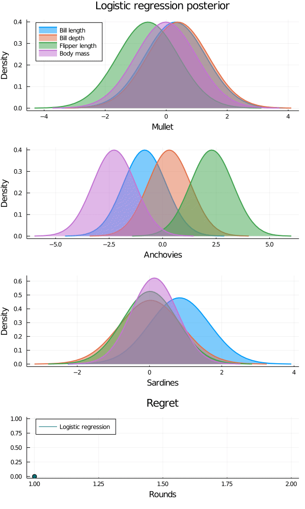
Figure 3: Animation of model posterior as it is presented with new data. The sardine model becomes quite confident, since it is the fish of choice for the Gentoo, which is easily recognised. However, the Adelie and Chinstrap features only differ significantly in the bill length, making them easy to mix up. This leads to higher uncertainty in the models for mullet and anchovies, which is their preferred fish.
Even though the mullet and anchovies models are struggling a bit, the regret of the logistic regression model is vastly superior to that of the Beta-Bernoulli model, as seen in the regret plot below. Recall that the optimal action is the one that minimised regret given the context, which is different than the one in the previous article (where we had no context). Hence, the regret plots are not directly comparable (we expect the Beta-Bernoulli to accumulate more regret for this problem since it is more difficult).

Figure 4: Comparing the regret of the two agents shows that the logistic regression model performs orders of magnitude better than the Beta-Bernoulli model. This is explained by the Beta-Bernoulli model simply discarding context information.
Ending notes
In these two articles we have seen how to treat recommender systems as multi-armed bandit problems, and covered some simple but very useful Bayesian methods for solving them. We saw how to directly infer a single best recommendation, and how to use context to personalise the recommendations further. But most importantly, we now have a way to automatically feed the penguins of Antarctica(!).
Now, there might be other problems out there which are more important to you than building recommender systems for penguins. Fortunately, multi-armed bandits are super versatile and can be used in a bunch of different domains, such as fraud detection, automated trading and active learning. They have also seen great success as replacements for A/B-testing. In contrast to the commonly used supervised learning they learn as they go and do not require periodical retraining, which makes them somewhat set-and-forget. (Given that continuous feedback is available). However, it is possible to run into issues such as covariate shift. One option to combat this is to use methods such as adaptive windowing to allow the model to track changing trends and behaviours. Another issue you might run into when updating the model continuously is that the parameter estimates fluctuate too much to give stable predictions. This can be combated by collecting observations and performing batch updates in a standard supervised learning fashion.
Thanks for reading. Don’t hesitate to shoot me an email if you have any comments or questions!