Me and my mates are big fans of craft beer, and from time to time organise our own beer tastings. Each participant gets to give a single score between 1 and 5 (half point increments are allowed) to each beer and afterwards we compare scores and see which beer came out on top. Sour beer and imperial stouts are some of our favourite styles, but this time we decided to do something different: A blind tasting with the cheapest lager we could find. In this article we are going to apply a Bayesian judge model to analyse the scores. Code available here.
The beer score data
The score data comprises a list of scores given by a specific judge to a specific beer. There are 7 beers and 4 judges. Here is a sample.
| judge | beer | score |
|---|---|---|
| A | 1 | 2.5 |
| A | 2 | 0.5 |
| B | 2 | 1.0 |
| B | 7 | 3.5 |
| C | 1 | 1.5 |
| C | 2 | 0.5 |
Since the dataset is small, we can easily get a good overview by scatter plotting it. We can for instance clearly see that beer 3 and 7 were the favourites while 5 and 6 were the least liked. Not a single beer scored above 3.5 though. Like I mentioned before, this is the cheapest stuff we could find.
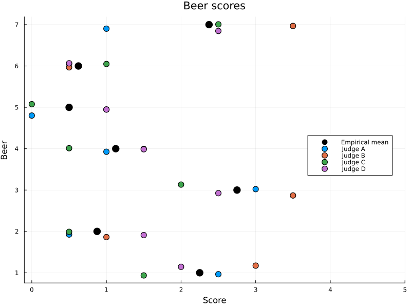
Figure 1: Beer score from each judge, with some jitter added to aid visualisation.
Now you might ask “What more is there to analyse? We have the individual scores and the empirical mean”. While that is true, I would argue that the scores assigned to each judge isn’t necessarily comparable in an apples-to-apples sense. Think of it this way: While each judge assigns scores on the same scale, they might have different latent scales. Judge A might use a symmetric scale where 2.5 is the average score, while Judge B might use a generous IMDB-like scale where even mediocre beer scores in the top 25 percentile. In addition to having different ideas of an “average score”, judges might also discriminate differently. Some judges might not discriminate a lot beween low and high quality beer, rating every beer about average, while others might discriminate more between good and bad and make use of the entire score scale. So, even though the empirical mean is far from useless, it might not actually answer the question of which beer is the best if the judges use different enough latent scales.
A Bayesian Judge Model
The goal of the analysis is going to be to tease apart the different latent quantities that give rise to the score \(S_i\) for beer \(i = 1 \dots N\). So let’s take a moment to think about what these are and how to model them. First off is the obvious quality \(Q_i\) of the beer, but we also established that the score depends on the judge who assigned it. Each judge \(j = 1 \dots J\) will be assumed to have an individual harshness \(H_j\) and discrimination \(D_j\). If we had information on individual beers or judges we could have included that as well, but this is all we got for this analysis. Before we interpret these quantities let us write out the full model to get the full context.
\begin{equation} \begin{split} Q_\mu & \sim \mathcal{N}(0, 1) \\ Q_\sigma & \sim \mathcal{N}^{+}(1) \\ D_\mu & \sim \mathcal{N}^{+}(1) \\ D_\sigma & \sim \mathcal{N}^{+}(1) \\ \sigma & \sim \mathcal{N}^{+}(1) \\ \\ D_j & \sim \mathcal{N}(D_\mu, D_\sigma) \\ H_j & \sim \mathcal{N}(H_\mu, H_\sigma) \\ \\ \mu_{i,j} & = D_j(Q_i - H_j) \\ S_{i,j} & \sim \mathcal{N}(\mu_{i,j}, \sigma^2) \end{split} \end{equation}
Where we use \(\mathcal{N}^{+}\) to denote a Half-Normal distribution. Note that we assume standardised data (zero mean, unit variance) for the priors. And here is a graphical representation of the above model.

Let us take a closer look at the equation \(\mu_{i,j} = D_j(Q_i - H_j)\) where most of the magic happens. The mean score \(\mu_{i,j}\) of a beer \(i\) given by judge \(j\) is the difference between the beer’s quality \(Q_i\) and the judge’s harshness \(H_j\), scaled by the judge’s discrimination \(D_j\). In other words, \(Q_i\) must be greater than \(H_j\) to score above average, and \(D_j\) “weights” this difference to produce the final score. A larger \(D_j\) means a judge discriminates more for small differences in \(Q_i\). Taken together, this means that a score given by a judge with a high \(H_j\) and low \(D_j\) indicates a larger \(Q_i\) than the same score from a judge with low \(H_j\) and high \(D_j\). Finally, we add hyperpriors to \(D_i\) and \(H_i\) to make use of partial pooling.
This model can be implemented in Turing.jl as follows. Notation closely follows the maths, except for the priors over \(H_j\) and \(D_j\), where we make use of non-centered parametrisation for computational reasons.
@model function judge_model(i, j, S, M, N)
    Hμ ~ Normal(0, 3)
    Hσ ~ truncated(Normal(0, 3), lower=0)

    Dμ ~ truncated(Normal(0, 3), lower=0)
    Dσ ~ truncated(Normal(0, 3), lower=0)

    # non-centered parametrisation
    Hz ~ filldist(Normal(0, 1), M)
    H = Hμ .+ Hz .* Hσ

    # non-centered parametrisation
    Dz ~ filldist(truncated(Normal(0, 1), lower=0), M)
    D = Dμ .+ Dz .* Dσ

    Q ~ filldist(Normal(0, 1), N)
    σ ~ Exponential(0.5)

    μ = D[j].*(Q[i] .- H[j])
    S .~ Normal.(μ, σ)
    return (;H, D)
end
Analysis
Fitting the model and plotting the posterior quality reveals the posterior mean to be very close to the empirical mean. But we do see some notable differences: beer 1, 3, 7 have higher estimated quality and beers 2 and 6 slightly lower. How come?

Figure 2: Posterior beer quality. The highest posterior density intervals (black lines) typically cover the individual scores, and the posterior mean is similar to the empirical mean.
The deviations from the empirical mean is explained by the posterior harshness and discrimination of the judges. In particular, Judge A and C have higher harshness and lower discrimination than judge B and D, so deviating scores from them are more impactful.
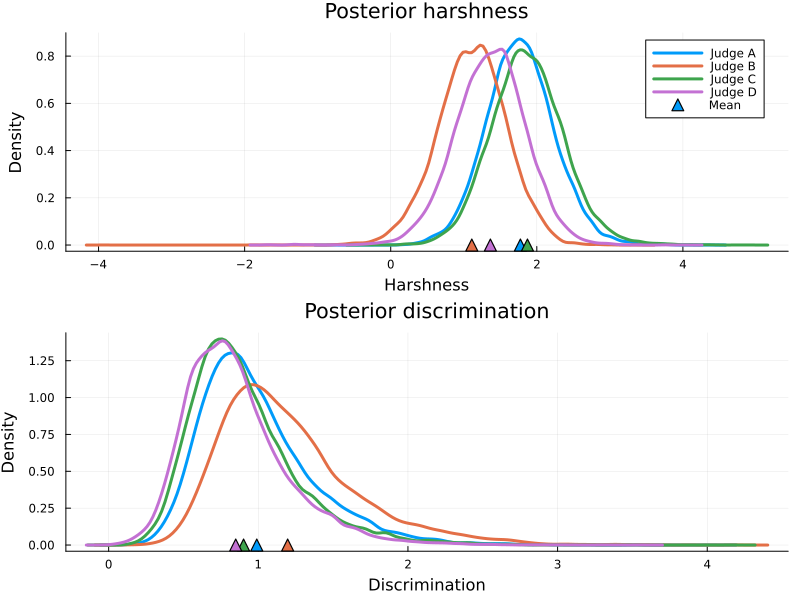
Figure 3: Posterior harshness and discrimination. Judge B is most willing to give high scores, while Judge A and Judge B are quite picky.
All in all, the posterior estimate doesn’t differ that much from the empirical estimate, which is explained by the fact that all judges have very similar characteristics. Our group did talk about our reviews during the tasting, so we are most likely seeing a regression-to-the-mean effect here. Should we have kept our scores a secret it is conceivable that the model would have uncovered different harshness/discrimination posteriors, which could have shifted the beer quality further.
Closing remarks
So there we have it. We have seen how to build and interpret a Bayesian judge model to score data. While we only modelled judge characteristics, this approach can easily be extended to include features of judges (e.g. nationality, age) and features of the object being scored (e.g. beer origin or style). And of course, this model can be used in any setting As always, the code is available here. Thanks for reading!