This is a follow-up post where we will see how to apply a normalizing flow model to learn the density of observed data. If you are not familiar with these models I recommend checking out the first part which explains how normalizing flows work and the math behind them. The promise of normalizing flows is that we can learn probability densities over our observations without having to model our entire domain by hand. We will see how to do this and how a trained model can be used to make predictions with quantifiable uncertainty. With that said, it’s time to roll up our sleeves and write some Python.
While it is common to show off generative models on images, we are going to tackle a simple problem where we can inspect the learned densities a bit easier. It is time to pull out the Iris dataset.
Normalizing flow(er)s
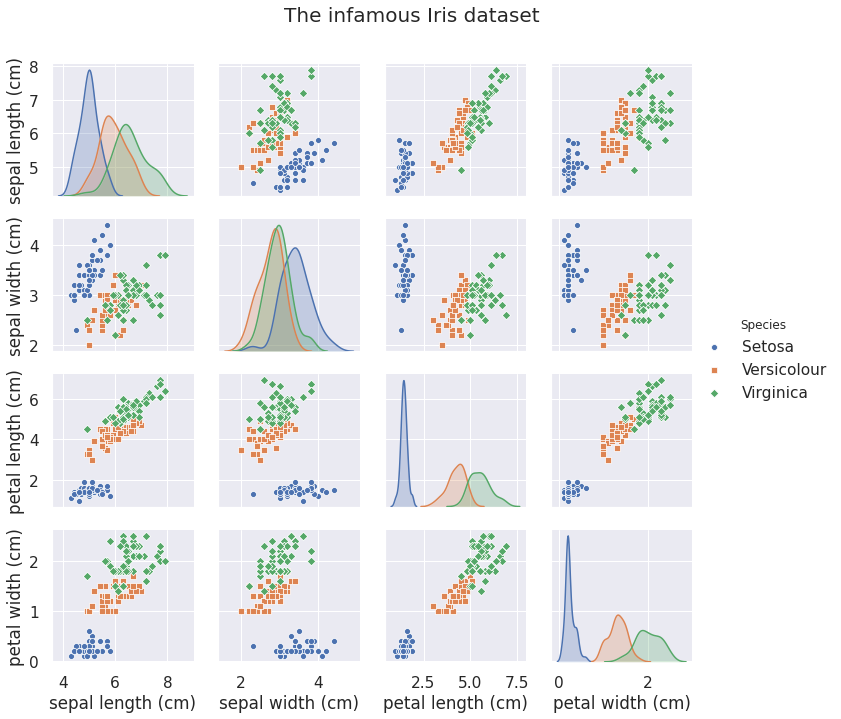
The Iris dataset does not need much of an introduction. In a nutshell it contains \(150\) observations comprising four different measurements from three flowers species.
  iris = sklearn.datasets.load_iris(as_frame=True).frame
  labels = {0: 'Setosa', 1: 'Versicolour', 2: 'Virginica'}
  iris['Species'] = iris.target.apply(lambda c: labels[c])
  true_species = torch.from_numpy(iris['target'].values)
  iris = iris.drop(columns='target')
We are going to learn the class conditional densities \(p(x \vert w_s) \) for each species \(s = \text{se}, \text{ve}, \text{vi}\). This is a simple dataset, so we do not need that many parameters to fit it. However, since we are using coupling layers, we need to use at least \(4\) layers to make sure all dimensions can interact.
Recall that our implementation already specifies the structure of coupling flows and affine transformations. To instantiate a model we need to supply a latent distribution \(p(z)\) and a list of flows \(f_n \circ \dots \circ f_2, \circ f_1\). We will let \( p(z) \) be a multivariate normal distribution. Each flow \(f_i\) needs a conditioner model \(\theta_i\) and a function to split the dimensions. We created a conditioner model in the last post, and since there is no natural order to the Iris features, we will simply use the order they appear in the data frame and split them in the middle. Lets create a function to assemble all these pieces into a new model.
  def affine_coupling_flows(
    data_dim: int,
    hidden_dim: int,
    num_hidden: int,
    num_params: int,
    num_flows: int,
    device: str
  ) -> nn.Module:

    def flow():
      split = partial(torch.chunk, chunks=2, dim=-1)
      theta = Conditioner(
        in_dim=data_dim // 2,
        out_dim=data_dim // 2,
        num_params=num_params,
        hidden_dim=hidden_dim,
        num_hidden=num_hidden
      )

      return AffineCouplingLayer(theta, split)

    latent = MultivariateNormal(
      torch.zeros(data_dim).to(device),
      torch.eye(data_dim).to(device)
    )
    flows = nn.ModuleList([flow() for _ in range(num_flows)])
    return NormalizingFlow(latent, flows)
For the hyper-parameters, we will use a model with \(5\) flows, and each flow will use a conditioner with a single hidden layers with \(100\) neurons. Since we use affine flows, the number of parameters are \(2\) (\(s\) and \(t\)).
  def simple_iris_model(device='cuda'):
   return affine_coupling_flows(
       data_dim=iris.shape[1]-1,
       hidden_dim=100,
       num_hidden=1,
       num_flows=5,
       num_params=2,
       device=device
     ).to(device)
Finally, let’s write some training logic. Training with affine
coupling layers can be a bit unstable, so we use learning rate decay
to aid convergence. Additionally, the regularization from mini-batching really
helps stabilize optimization so we will use a mini-batch of 32. With
that said, we can simply plug in the AdamW optimizer and train the model
by minimizing the negative log probability of the data.
    def train(
      model: nn.Module,
      train_loader: DataLoader,
      num_epochs: int,
      args
    ) -> torch.Tensor:

      def _train(epoch, log_interval=50):
	model.train()
	losses = torch.zeros(len(train_loader))
	for i, x in enumerate(train_loader):
	  optimizer.zero_grad()
	  loss = -model.log_prob(x.to(device)).mean()
	  loss.backward()
	  losses[i] = loss.item()
	  optimizer.step()

	return losses.mean().item()

      def log_training_results(loss, epoch, log_interval):
	if epoch % log_interval == 0:
	  print("Training Results - Epoch: {}  Avg train loss: {:.2f}"
		.format(epoch, loss))

      optimizer = torch.optim.AdamW(model.parameters(), lr=args['lr'])
      num_steps = len(train_loader)*num_epochs
      scheduler = StepLR(
	  optimizer,
	  step_size=args['lr_decay_interval'],
	  gamma=args['lr_decay_rate']
      )

      train_losses = []
      for epoch in range(num_epochs+1):
	loss = _train(epoch)
	log_training_results(loss, epoch, log_interval=100)
	train_losses.append(loss)
	scheduler.step()

      return train_losses


    def train_new_model(data, num_epochs, args):
      np.random.seed(1)
      model = simple_iris_model()
      loader = partial(DataLoader, batch_size=32, shuffle=True)
      loss = train(
	model=model,
	train_loader=loader(data),
	num_epochs=num_epochs,
	args=args
      )

      return model, loss
Now everything is in place to train the models!
  args={'lr_decay_interval': 400,
        'lr_decay_rate': .3,
        'lr': 1e-3}

  def target_class(species: str) -> torch.Tensor:
    x = iris[iris['Species'] == species].drop(columns='Species')
    return torch.from_numpy(x.values).float()

  device = 'cuda:0'
  classes = list(labels.values())
  train_with_args = partial(train_new_model, num_epochs=2000, args=args)
  model_se, loss_se = train_with_args(target_class(classes[0]))
  model_ve, loss_ve = train_with_args(target_class(classes[1]))
  model_vi, loss_vi = train_with_args(target_class(classes[2]))
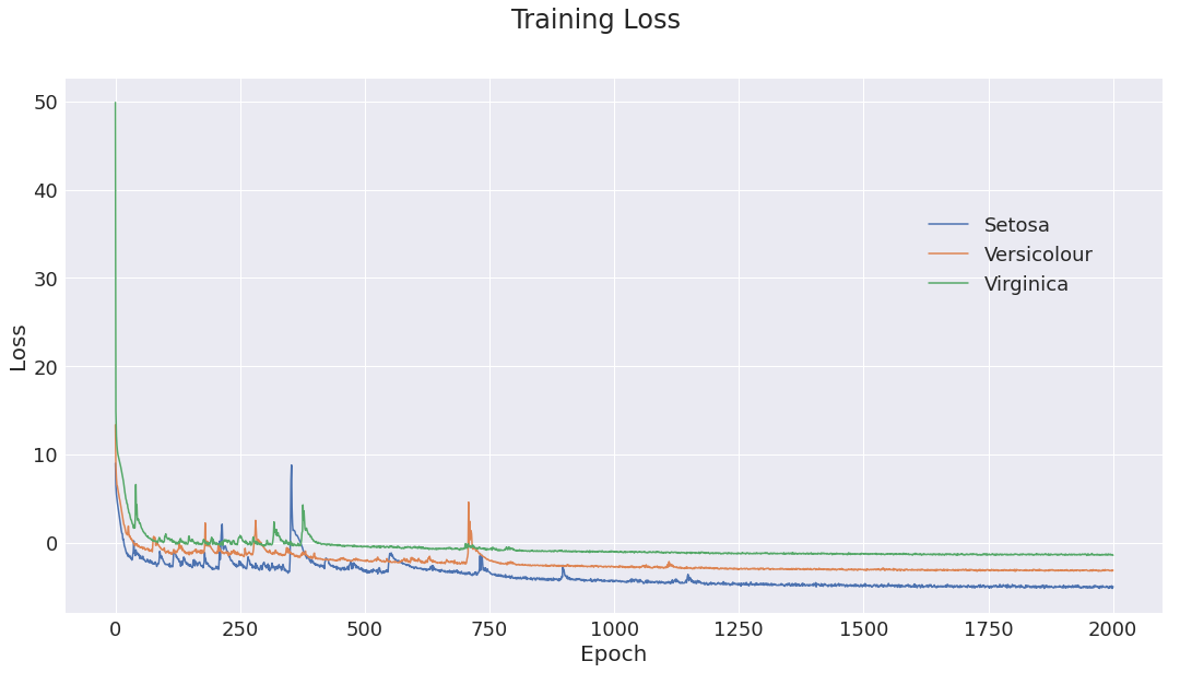
Figure 1: Training loss for the three class models. Initial optimization is somewhat unstable, but as learning rate decays, optimization converges to a good minima.
Optimization successfully converges. So how good is the fit? Has the model learned the structure of the data?
Assessing model performance
The negative log likelihood tells us whether the model trains or not, and gives us a way of comparing different hyper-paremeter choices or models. Unfortunately, it does not tell us much about how good the model actually is in quantities we care about. So to assess model performance we simulate from the learned densities and compare with true observation.
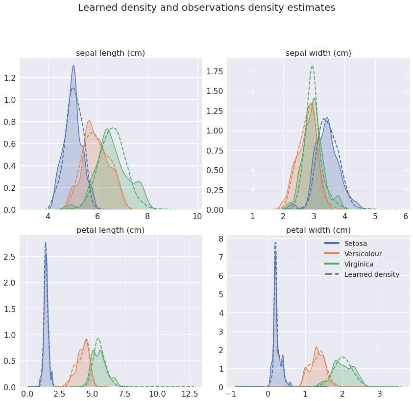
Figure 2: Kernel density estimate of observations and (2000) simulations per class. The model learns quite complex non-Gaussian densities and faithfully captures the target distributions.
Comparing the densities shows that the model has successfully learned the class conditional distributions. Great!
We did not put aside any data for testing out-of-sample performance, but as a sanity check we can check the in-sample accuracy for the model. We predict the species \(\hat{s}\) for new observations \(\tilde{x}\) by treating prediction as a model selection problem and by selecting the most probable model
\[ \hat{s} = \underset{s}{\mathrm{argmax\,}} p(w_s \vert \tilde{x}) = \underset{s}{\mathrm{argmax\,}} p(\tilde{x} \vert w_s)p(w_s) \]
using a discrete uniform prior \(p(w_s)\). Some observations have so small probabilities that we get nan
values. We should interpret this as the model considering these
observations extremely unlikely under the current class conditional density.
We deal with these values by replacing them with \(-\infty\).
    def class_probs(x, class_models):
      with torch.no_grad():
	log_probs = torch.stack([
	  m.log_prob(x.float().cuda()).cpu()
	  for m in class_models
	])

	log_probs[torch.isnan(log_probs)] = -math.inf
	probs = log_probs.exp()
	probs /= probs.sum(0)
	return probs

    def predict(class_probs):
	return class_probs.argmax(0)

    def accuracy(y, y_hat):
      return y.eq(y_hat).float().mean().item()

    x = torch.from_numpy(iris.iloc[:, :-1].values)
    probs = class_probs(x, class_models=[model_se, model_ve, model_vi])
    pred_species = predict(probs)
    print(f'Model accuracy: {accuracy(true_species, pred_species)}')
Model accuracy: 1.0
The model perfectly classifies all the observations. Excellent! Since we are using a probabilistic model, we can easily find which observations the model was least certain about by computing the entropy of \(p(s\vert \tilde{x})\).
  def entropy(x):
    return torch.from_numpy(scipy.stats.entropy(x.numpy()))

  x_uncertain = torch.topk(entropy(probs), k=5, dim=0)
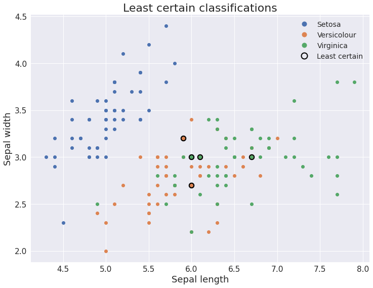
Figure 3: Sepal width vs sepal length with the least certain classifications highlighted. As expected, the model is less certain about the very similar observations from the Versicolour and Virginica species.
This makes perfect sense to us, since the Versiculour and Virginica species are very similar. But this is only one thing we can do with a distribution. Should the model be presented with rubbish data, we will be able to automatically detect this, since none of the class conditional densities will give it a high likelihood. And we were able to achieve all this without explicitly modeling our domain using analytical probability distributions.
Some notes on normalizing flows
In this article we applied the model we implemented in the first part to the Iris dataset and successfully learned the class conditional densities. We also covered how these models can be used to classify new observations and how they make it super easy to quantify model uncertainty and detect outliers. When playing around with hyper-parameters for training I often experienced spikes in the loss curves for fairly standard learning rates around \(1e^{-3}\). Using a smaller learning rate together with learning rate decay and smaller batch sizes helped stabilize the optimization and lead to successful training.
I hope you have enjoyed these two post about normalizing flows. They are a really interesting model class, and not as esoteric as people might think. As we have seen, they are quite capable of solving everyday machine learning problems. And while they have a few more moving pieces than a simple classification network, they can be used in a black-box fashion like any other network.
Comments or questions? Shoot me an email!